Analytics on Wind Turbine SCADA Data
- Each wind turbine issues SCADA packets at 10 minutes intervals
- Each wind turbine, according to the OEM’s specs, have different system parameters found within SCADA packets
- Even small wind farm generates tens of millions of packets per month
Analytics Backend
- SCADA packets are aggregated into a mySQL database
- Ensemble of algorithms performed using Wolfram Programming Language or Mathematica (Cloud)
- DataNotes created for Web viewing
- DataNotes are unital standalone computational structures focused on specific analytical aspect of specific data
Visualization
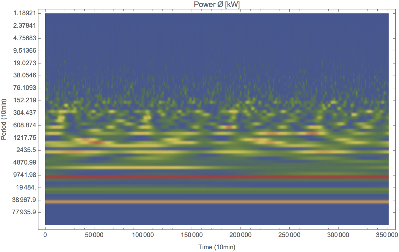
Wavelet Signal Decomposition
Partial data to show strong periodicity onwards of 76 units of time.
Strong 300 to 450 periods (10 mins).
Predict with Variable Selection
Each wind turbine has large set of parameters governing its operations and dynamics.
Algorithm searches for the most optimal set of input variables to produce a Predict function of highest accuracy:
https://en.wikipedia.org/wiki/Feature_selection
Parameters={“Rotar speed”,”Wind speed”,”Wind direction”,”Nacelle Position”,”Power”,”Generator RPM”,”Ambient temperature”}
From the above list of variables 1 to 7 could be chosen for input vector, combinatorically, to predict another parameter (in the next time unit which is 10 mins).
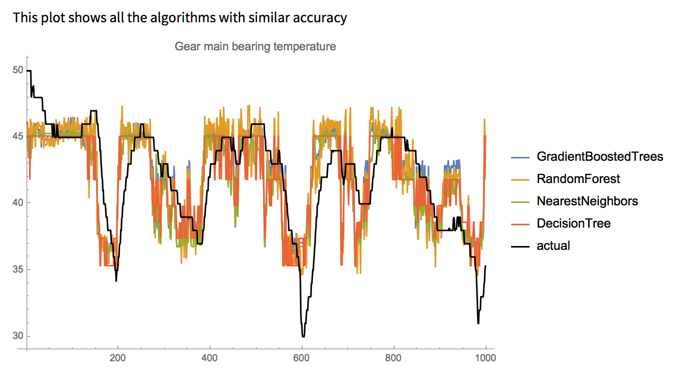
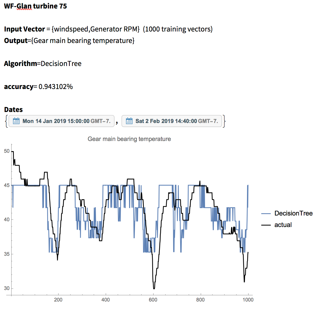
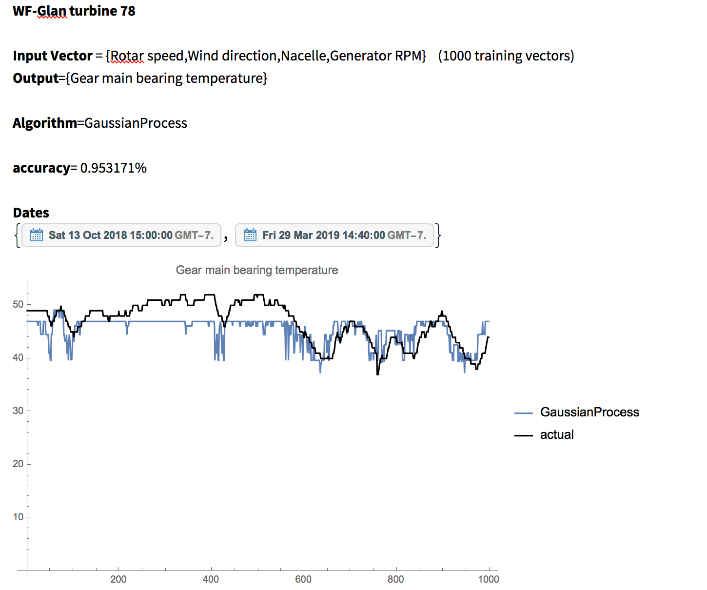
Prediction for “Gear main bearing temperature” parameter, as in the case of the below trials. Idea is if other parameters could be used to predict “Gear main bearing temperature” without it appearing in the training set.
Multiple algorithms also variated along side the input parameters to search for the best combination of algorithms and input vectors:
Algorithms={“GradientBoostedTrees”,”RandomForest”,”NearestNeighbors”,”DecisionTree”,”GaussianProcess”}
All combinations of the input parameters, total 127.
Given the 5 algorithms total combinations of 5×127=635.
Complexity
Each search for the optimal input vectors and predict algorithm took 10-15 mins of time on a 64 cpu core Linux server with 1 TB of physical memory. Approximately 40G of memory consumption and all 64 cpu cores 100% pegged.
For a wind farm of 100 turbines roughly 24 hours needed to search for the optimal input vectors and predict algorithms.
Each plot above takes about 15 mins of computations on all 64 cpu cores.
On smaller machine the above is unattainable since 1 run of the algorithm would take 8-10 hours!
{{“rotarspeed”}, {“windspeed”}, {“Wind direction”}, {“nacelle”},
{“power”}, {“Generator RPM”}, {“Ambient temperature”}, {“rotarspeed”,
“windspeed”}, {“rotarspeed”, “Wind direction”}, {“rotarspeed”,
“nacelle”}, {“rotarspeed”, “power”}, {“rotarspeed”,
“Generator RPM”}, {“rotarspeed”,
“Ambient temperature”}, {“windspeed”,
“Wind direction”}, {“windspeed”, “nacelle”}, {“windspeed”,
“power”}, {“windspeed”, “Generator RPM”}, {“windspeed”,
“Ambient temperature”}, {“Wind direction”,
“nacelle”} … {“rotarspeed”, “windspeed”, “nacelle”,
“power”, “Generator RPM”, “Ambient temperature”}, {“rotarspeed”,
“Wind direction”, “nacelle”, “power”, “Generator RPM”,
“Ambient temperature”}, {“windspeed”, “Wind direction”, “nacelle”,
“power”, “Generator RPM”, “Ambient temperature”}, {“rotarspeed”,
“windspeed”, “Wind direction”, “nacelle”, “power”, “Generator RPM”,
“Ambient temperature”}}
Sample DataNote
Note: Ensemble of algorithms performed on larger multi-cpu servers to search for the most optimized algorithm from the bunch e.g. Gaussian Process was found to be the best Predict function on that specific data for the specific interval of time. This search might yield different candidate for different dates.
Similarity
Currently the Similarity algorithm is inter-turbine measuring how similar the turbine behaves apropos of its past historical data.
In the future development we shall definitely provide intra-turbine similarity to compare turbines.
Interactive CloudNote
Classifier
At the helm of the management of wind farms, daily computed Classifiers are provided with mobile web access.
Turbine id allows for its classifier access. Number of mix-mode parameters could be entered by the management into the input boxes of the classifier web interface.
Upon pressing the button Classify! A Class is computed accordingly.
In the CloudNote below Rotation Speed and Wind Speed and Nacelle Position are entered by the user and in return Power Level Classes issued from A (high power) to F (no power) and gradatations in between by B, C and D letters representing classes.
Interactive CloudNote
Clusters
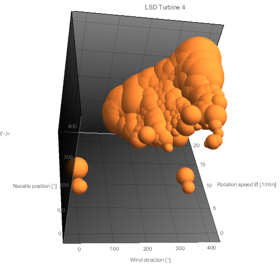
Density Clusters
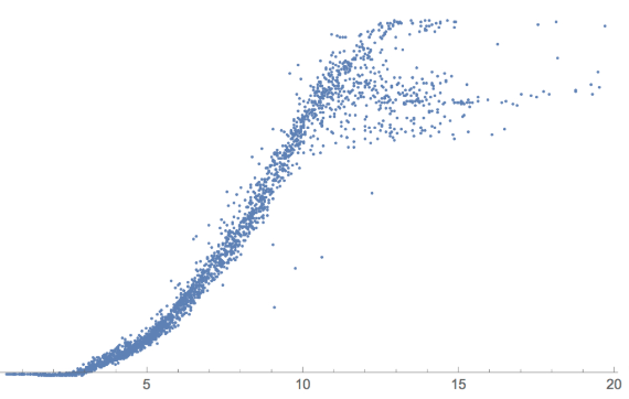
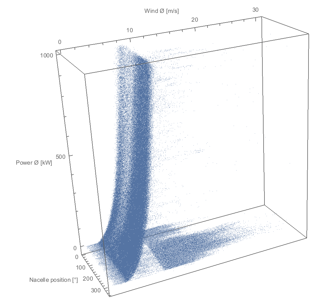
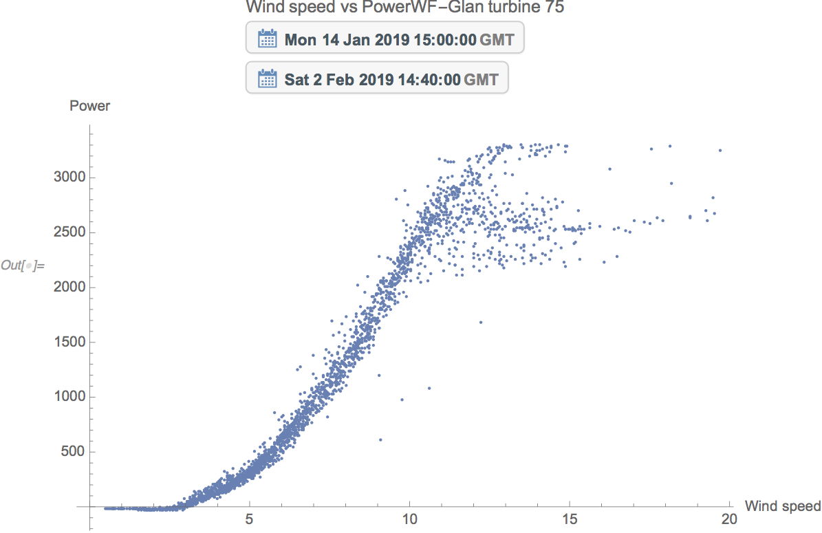
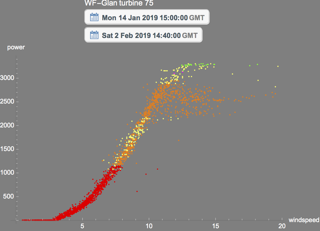
DBSCAN or Density-based spatial clustering of applications with noise is a useful type of clustering suitable for measuring and viewing Power scatter plots of wind turbines that might in general all look the same but the density clustering render which part of the power curve was occupied by the data points most.
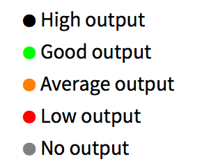
The following blue-ish scatter plot does not tell us much about the clustering of the power output but the corresponding density cluster with color code tells us where the turbine spent most of its output namely Red most dense Yellow least and the other colors gradations in between.
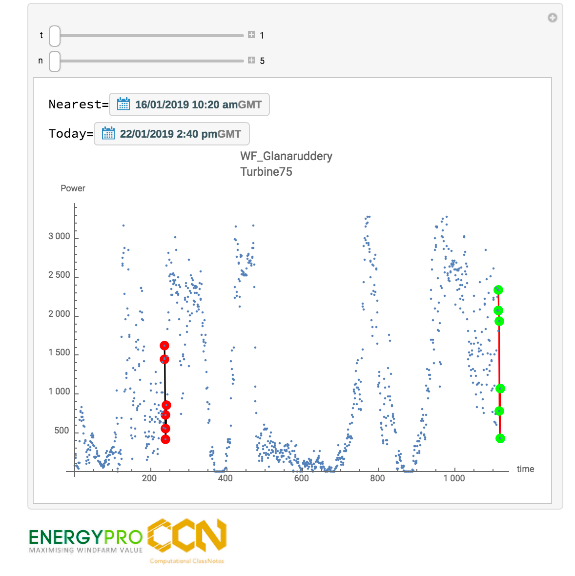
K-NN-G
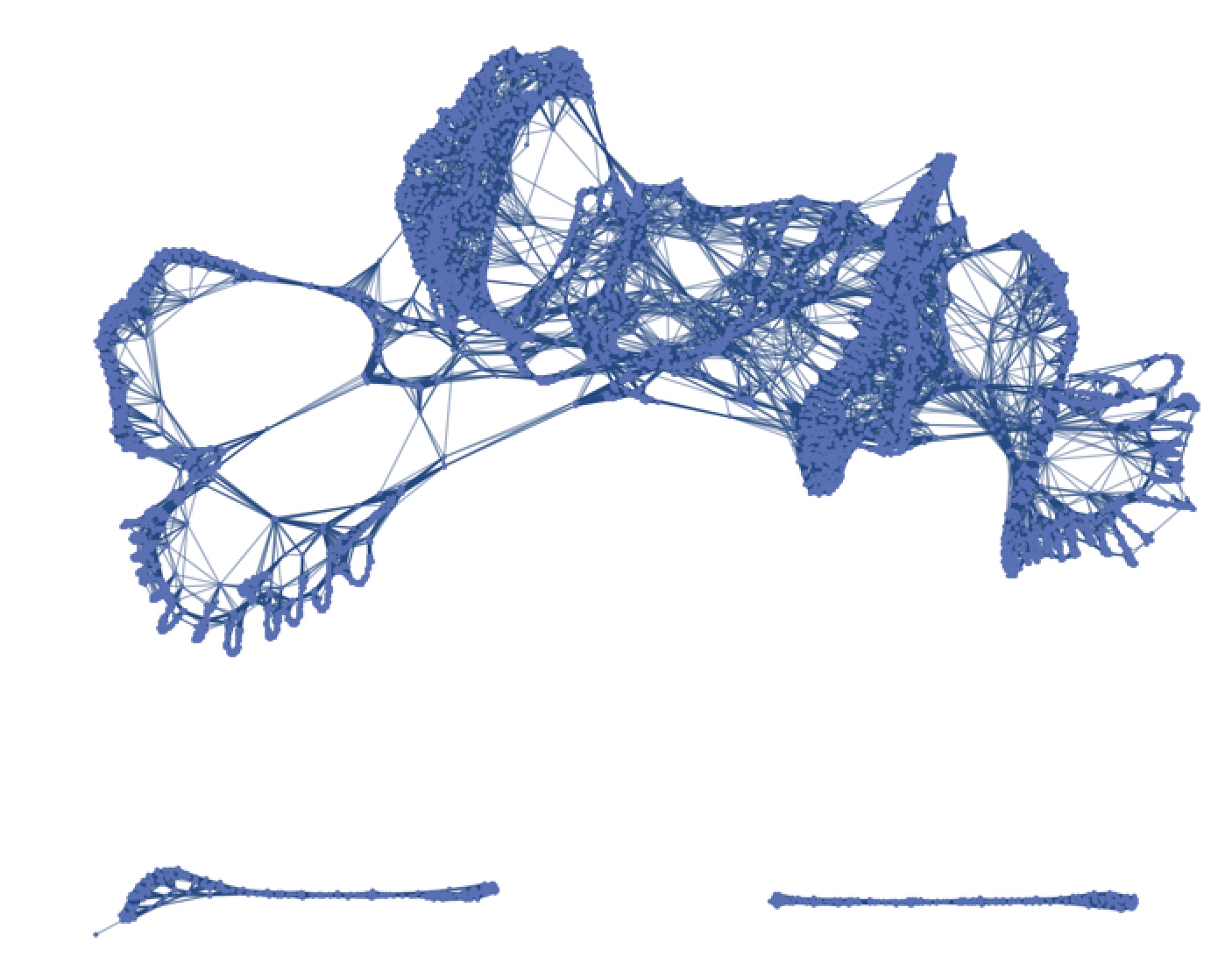
The nearest neighbor graph (NNG) for a set of n objects P in a metric space (e.g., for a set of points in the plane with Euclidean distance) is a directed graph with P being its vertex set and with a directed edge from p to q whenever q is a nearest neighbor of p (i.e., the distance from p to q is no larger than from p to any other object from P).
Each node is a scanned data point for a singl turbine. .
Simple color coding allows for visual inspection.
Highlighted number is the accuracy for Classification of output in this graph.

Legend
Mouse-over pops the tooltip including all the pertinent data.
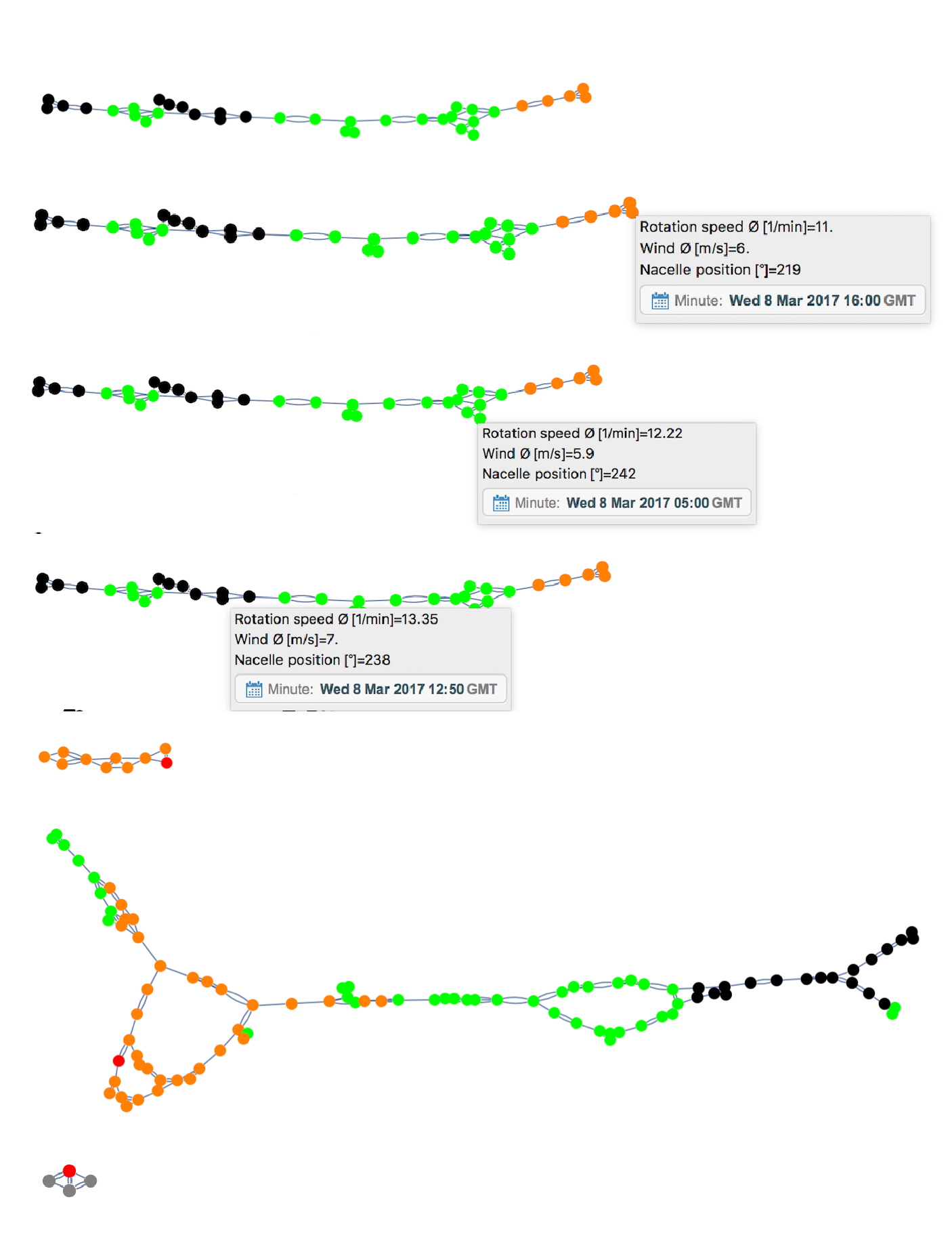
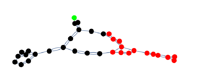
Ideal graphs

Ambiguous
© Present-2019, Computational ClassNotes